Welcome to the Build-A-Neuron Workshop! In here, we don’t simply build neurons — we build life-long friends!
So what are we waiting for? Let’s begin!
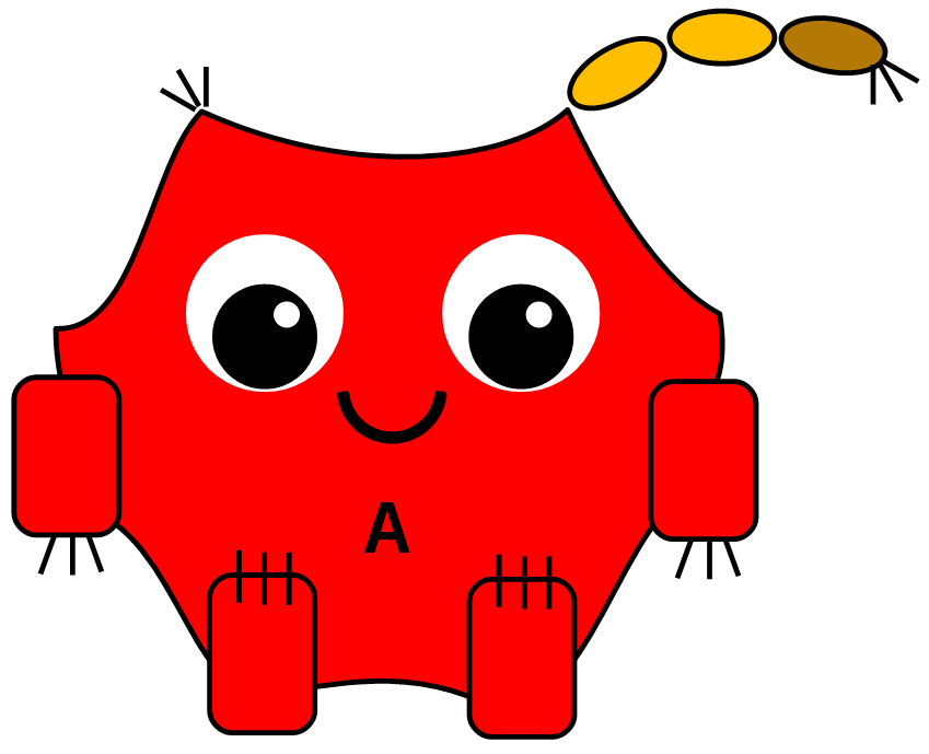
We’ll name our first neuron, Alice:
main(  )
{
    alice = new Neuron(  );
}
/* separate source file */
class Neuron
{
…
}Innit she just the sweetest thing you ever seen?
Oh, look, she wants to give you a hug! Awwwww … .
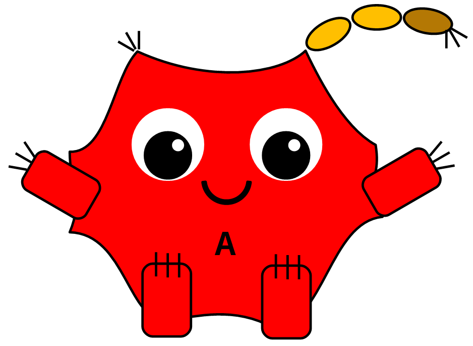
But she ain’t just cute n’ cuddly! She’s capable of so much more — so let’s put her to work!
There Are Lines You Just Don't Cross
We’ll magically create some training data for her. Abby Cadabby!
main(  )
{
    alice = new Neuron(  );
    hvm = new SyntheticData(  );
    hvm.collect_data
        ( "train_hatfields_vs_mccoys.txt" );

    …
}
/* separate source file */
class SyntheticData
{
collect_data( filename )
{ … }
…
}TM( ) = ?Hatfield → target variable is 1
McCoy → target variable is -1
| Data Point | Feature 1 | Feature 2 | Target Variable | Label |
|---|---|---|---|---|
| dpH1 | -5 | -6 | 1 | Hatfield |
| dpH2 | -7 | -3 | 1 | Hatfield |
| dpH3 | -5 | -2 | 1 | Hatfield |
| dpH4 | -6 | 3 | 1 | Hatfield |
| dpH5 | -4 | 4 | 1 | Hatfield |
| dpH6 | -3 | -4 | 1 | Hatfield |
| dpH7 | -2 | 2 | 1 | Hatfield |
| dpH8 | -1 | 7 | 1 | Hatfield |
| dpH9 | 0 | 5 | 1 | Hatfield |
| dpH10 | 2 | 8 | 1 | Hatfield |
| dpH11 | -7 | 1 | 1 | Hatfield |
| dpH12 | -9 | -2 | 1 | Hatfield |
| dpH13 | -7 | -8 | 1 | Hatfield |
| dpH14 | -7 | -10 | 1 | Hatfield |
| dpH15 | -4 | 1 | 1 | Hatfield |
| dpH16 | 3 | 10 | 1 | Hatfield |
| dpH17 | 0 | 2 | 1 | Hatfield |
| dpH18 | 1 | 6 | 1 | Hatfield |
| dpH19 | -4 | -6 | 1 | Hatfield |
| dpH20 | -2 | 9 | 1 | Hatfield |
| dpM1 | -2 | -8 | -1 | McCoy |
| dpM2 | 1 | -4 | -1 | McCoy |
| dpM3 | 4 | -6 | -1 | McCoy |
| dpM4 | 2 | -1 | -1 | McCoy |
| dpM5 | 7 | -2 | -1 | McCoy |
| dpM6 | 5 | 0 | -1 | McCoy |
| dpM7 | 3 | 4 | -1 | McCoy |
| dpM8 | 5 | 4 | -1 | McCoy |
| dpM9 | 6 | 7 | -1 | McCoy |
| dpM10 | 5 | 9 | -1 | McCoy |
| dpM11 | 2 | -8 | -1 | McCoy |
| dpM12 | 4 | 7 | -1 | McCoy |
| dpM13 | 6 | 2 | -1 | McCoy |
| dpM14 | -4 | -9 | -1 | McCoy |
| dpM15 | -1 | -5 | -1 | McCoy |
| dpM16 | 8 | 8 | -1 | McCoy |
| dpM17 | 6 | -8 | -1 | McCoy |
| dpM18 | 7 | 10 | -1 | McCoy |
| dpM19 | 0 | -6 | -1 | McCoy |
| dpM20 | 1 | -10 | -1 | McCoy |
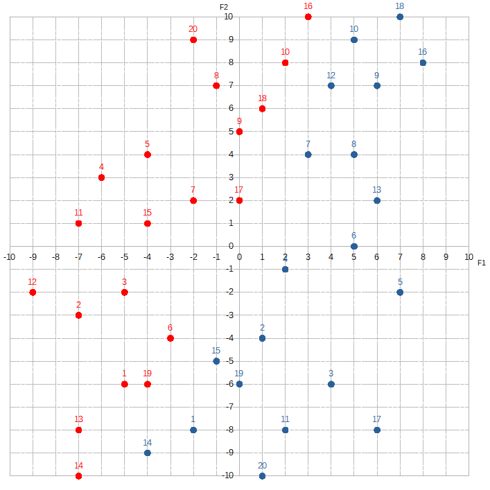
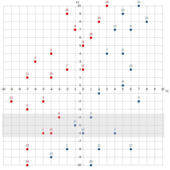
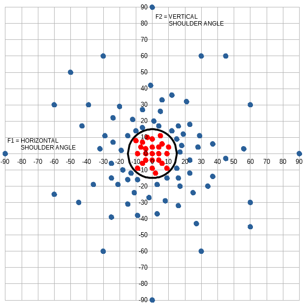
There are two features in this set ( F1 and F2 ) and two labels ( Hatfield and McCoy ). We’re going to train Alice to distinguish between the red dots and the blue dots. Since this is a classification problem, we’ll simplify both the computation and the code by limiting the target values to just 1 or -1.
However, because Alice was created only moments ago, we do need to be mindful about overwhelming her. So what should we do? Well, since we’re still in the Build-A-Neuron Workshop, let’s build her some friends!
main(  )
{
    alice = new Neuron(  );
    bob = new Neuron(  );
    carol = new Neuron(  );

    friends = { bob, carol };

    hvm = new SyntheticData(  );
    hvm.get_data( "train_hatfields_vs_mccoys.txt" );

    …
}

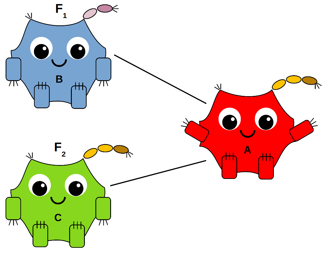
Bob will be responsible for learning the first feature of each data point, F1, while Carol will be responsible for the second, F2. Alice will take the information from her friends and use it to decide whether the label should be Hatfield or McCoy:
main(  )
{
    alice = new Neuron(  );
    bob = new Neuron(  );
    carol = new Neuron(  );

    friends = { bob, carol };

    hvm = new SyntheticData(  );
    hvm.collect_data
        ( "train_hatfields_vs_mccoys.txt" );
    dp = hvmSet.firstDataPoint;

    bob.collect_feature_value( dp.f1 );
    carol.collect_feature_value( dp.f2 );

    alice.collect_target_value( dp.trgtVal );
    alice.collect_label( dp.label );
    alice.collect_feature_values_from( friends );

    …
}
/* separate source file */
class Neuron
{
feature;
trgtVal;
label;
collect_feature_value( value )
{
feature = value;
}
collect_target_value( value )
{
trgtVal = value;
}
collect_label( value )
{
label = value;
}
collect_feature_values_from
( neurons )
{ … }
…
}
Since their roles are slightly different, let’s create two types of neurons — an input neuron and an output neuron.
main(  )
{
    alice = new OutputNeuron(  );
    bob = new InputNeuron(  );
    carol = new InputNeuron(  );

    friends = { bob, carol };

    hvm = new SyntheticData(  );
    hvm.collect_data( "train_hatfields_vs_mccoys.txt" );
    dp = hvmSet.firstDataPoint;

    bob.collect_feature_value( dp.f1 );
    carol.collect_feature_value( dp.f2 );

    alice.collect_target_value( dp.trgtVal );
    alice.collect_label( dp.label );
    alice.collect_feature_values_from( friends );

    …
}
/* separate source file */
class InputNeuron
{
feature;
retrieve_feature_value( value )
{
feature = value;
}
…
}/* separate source file */
class OutputNeuron
{
trgtVal;
label;
collect_target_value( value )
{
trgtVal = value;
}
collect_label( value )
{
label = value;
}
collect_feature_values_from( inputNeurons )
{ … }
…
}Alice’s main task is to find a line that separates the Hatfields from the McCoys.
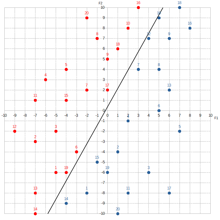
With this line, she will be able to classify new dots easily. If a new dot appears above the line, she will label it Hatfield. If it appears below, she will label it McCoy. The line equation takes the form, w1*F1 + w2*F2 + w0.
W1 and w2 are called weights, and w0 is called the bias. They’re multiplied to the values of their corresponding features. These weights tell Alice just how important the information she’s being given is.

A lower weight tells Alice that the information is not that important, while a higher weight signals that closer attention is warranted.
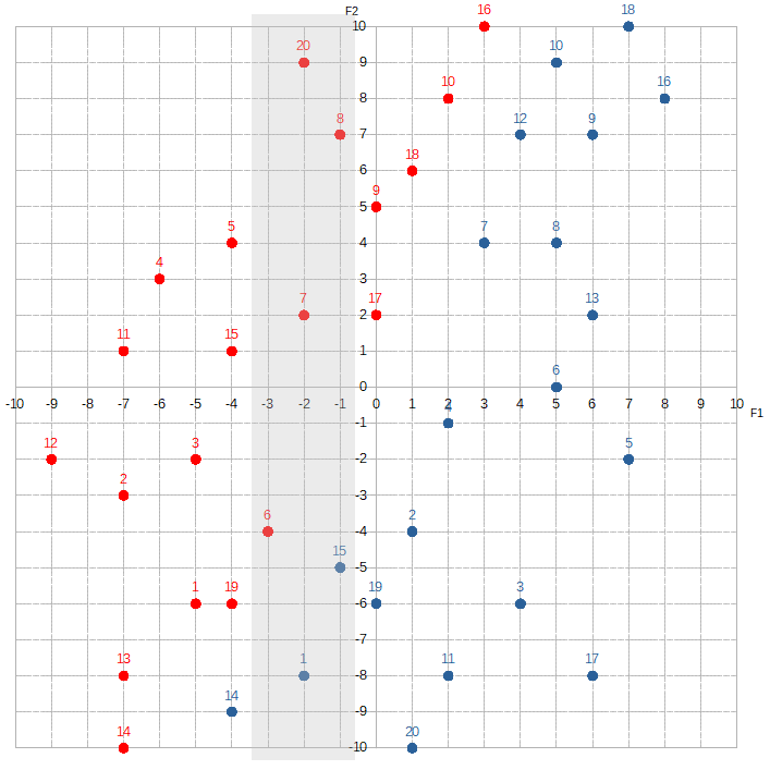
What makes a feature more important than another essentially depends on how much the composition of red dots to blue dots changes as the value of each feature changes. For example, let’s look at the section where F1 is between -3 and -1.
F1 is between 1 and 3: 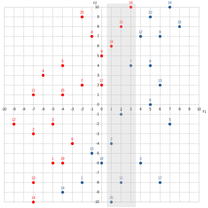
The proportion of red dots to blue dots changes dramatically. The McCoys now seem to “occupy” much more of this region than the Hatfields. This kind of information is extremely valuable to Alice. By knowing F1, she can dramatically increase her odds of correctly predicting the label. If she sees that F1 equals, say, -3, -2, or -1, she would guess Hatfield. If she sees F1 is 1, 2, or 3, she would guess McCoy. To signify F1‘s importance, Alice would assign a relatively high value to w1.
Contrast this with F2:
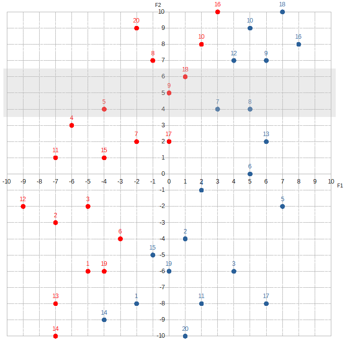
Where F2 is between 4 and 6, the Hatfields seem to sorta have a slight edge over the McCoys. If we shift over ten spots to where F2 is between -4 and -6:
The McCoys now seem have the edge — maybe. Knowing the value of F2 doesn’t help Alice much. She would assign a relatively low number to w2.
F2 is kind of like you receiving a text from your friend to meet him in the parking lot of a strip mall in some podunk town. Unfortunately, there are thousands upon thousands of podunk towns dotted across the United States. This text doesn’t help you figure out where you need to go. F1, on the other hand, is like your friend texting you to meet him in the Observatory of the Freedom Tower, or texting you to meet him at the base of the Gateway Arch. With this type of very specific information, you can pinpoint to within feet of exactly where you need to go.
The line equation may vaguely remind you of another equation that you learned back in elementary school: y = mx + b, where m is the slope of the line and b is the y-intercept. Well, that’s because they’re both one and the same! W1 and w2 are components of slope m — and w0 is similar to the y-intercept. There’s a reason why they teach us this stuff in grade school!
Changing w1 or w2 allows Alice to adjust the angle of the line clockwise or counter-clockwise:
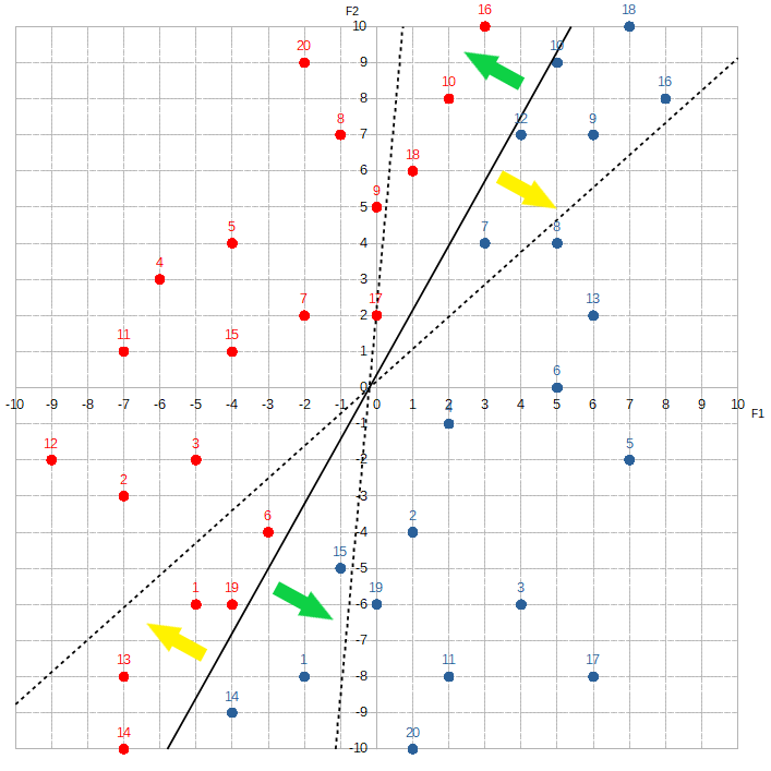
w1 increases or w2 decreases.Yellow arrows show direction when
w1 decreases or w2 increases.Changing w0 allows Alice to move the line vertically or horizontally:
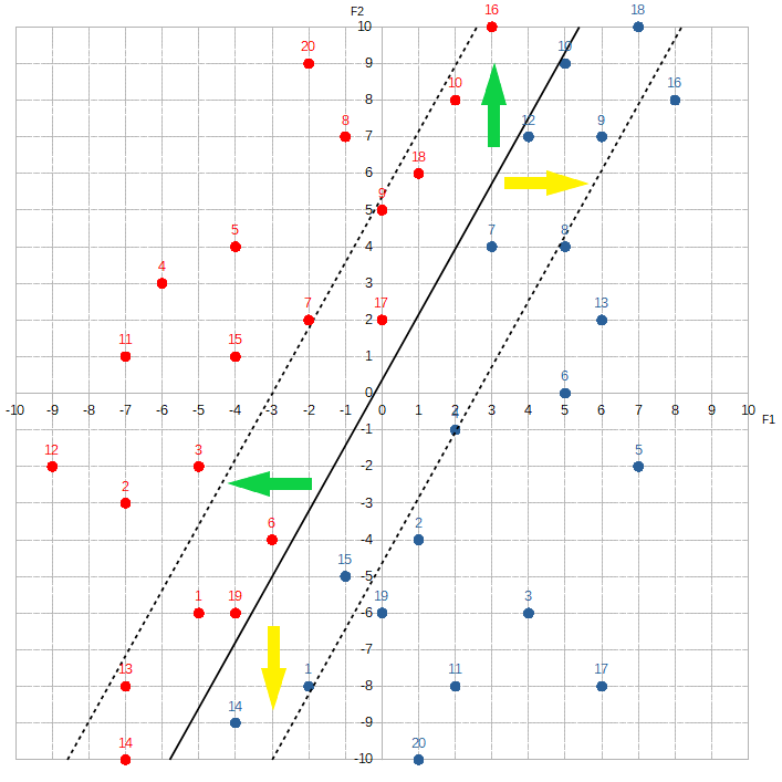
w0 increases.Yellow arrows show direction when
w0 decreases.Alright, now that we’ve covered the tools that Alice has at her disposal, let’s begin the learning process!
The first step is the most critical, which is to set the line equation equal to zero: w1*F1 + w2*F2 + w0 = 0. What this means is that we want to modify the weights and the bias in such a way that any data point that falls on the line will output a target value of zero. The reason why we want to do this is because this necessarily forces the data points that fall above the line to output predicted target values greater than zero, and the data points that fall below the line to output predicted target values less than zero.
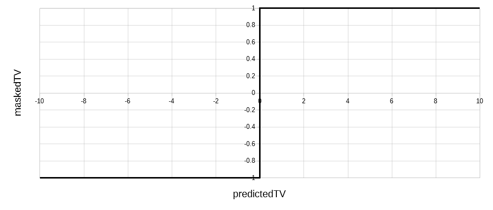
This vastly simplifies the classification problem for Alice. She doesn’t need to plot out a graph or do anything complicated. All she needs to do is look at the predicted target value. Since the actual target value is limited to 1 or -1, we’ll simplify things even further by masking the predicted target value with a step function:
main(  )
{
    …
    dp = hvm.firstDataPoint;

    bob.collect_feature_value( dp.f1 );
    carol.collect_feature_value( dp.f2 );

    alice.collect_target_value( dp.trgtVal );
    alice.collect_label( dp.label );

    alice.calc_predicted_target_val( friends );
    alice.calc_masked_target_val(  );
    alice.assign_predicted_label( "Hatfield", "McCoy" );

    …
}
/* separate source file */
class InputNeuron
{
feature;
weight;
collect_feature_value
( value )
{
feature = value;
}
…
}/* separate source file */
class OutputNeuron
{
trgtVal;
label;
bias;
prdctdTrgtVal;
maskedTrgtVal;
prdctdLbl;
collect_target_value( value )
{
trgtVal = value;
}
collect_label( value )
{
label = value;
}
calc_predicted_target_val( inputNeurons )
{
collect_feature_values_from( inputNeurons );
collect_weights_from( inputNeurons );
prdctdTrgtVal = sum( weights * features ) + bias;
}
calc_maskedTrgtVal( )
{
if ( prdctdTrgtVal > 0 )
maskedTrgtVal = 1;
else
maskedTrgtVal = -1;
}
assign_label( lbl1, lbl2 )
{
if ( maskedTrgtVal = 1 )
prdctdLbl = lbl1;
else
prdctdLbl = lbl2;
}
collect_feature_values_from( inputNeurons )
{ … }
collect_weights_from( inputNeurons );
{ … }
…
}Masking means exactly that. We’re changing the “appearance” of the predicted target value. This way, if the predicted target value is greater than 0, then the masked target value is 1, and Alice will label the datapoint Hatfield. If it’s less than 0, then the masked value is -1, and she’ll label it McCoy.
Since Alice has no idea what the correct weights are yet, let’s start her off with some arbitrary values.
main(  )
{
    …
    dp = hvm.firstDataPoint;

    bob.collect_feature_value( dp.f1 );
    carol.collect_feature_value( dp.f2 );

    alice.collect_target_value( dp.trgtVal );
    alice.collect_label( dp.lbl );

    bob.set_weight( -0.5 );
    carol.set_weight( 0.5 );
    alice.set_bias( 0.0 );

    alice.calc_predicted_target_val( friends );
    alice.calc_masked_target_val(  );
    alice.assign_predicted_label( "Hatfield", "McCoy" );

    …
}
/* separate source file */
class InputNeuron
{
feature;
weight;
collect_feature_value( value )
{
feature = value;
}
set_weight( value )
{
weight = value;
}
…
}/* separate source file */
class OutputNeuron
{
trgtVal;
label;
bias;
prdctdTrgtVal;
maskedTrgtVal;
label;
set_bias( value )
{
bias = value;
}
…
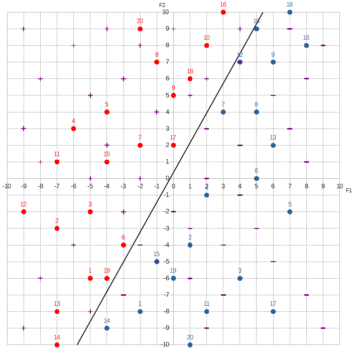
}Which means the trained model she’ll be using is: -0.5 * F1 + 0.5 * F2 + 0.0.
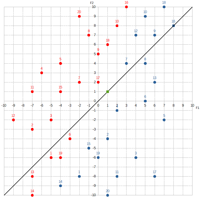
The black line marks all the points whose target values equal zero under this trained model. We can check this with the green dot that is sitting on the line, by plugging in it feature values ( F1 = 1, F2 = 1 ) into the equation:
tvgreen = -0.5 * F1 + 0.5 * F2 + 0
tvgreen = -0.5 * 1  + 0.5 * 1 + 0
tvgreen =    -0.5   +   0.5   + 0
tvgreen = 0
With everything initialized, Alice can start learning! Let’s see how she does with the first data point ( F1 = -5, F2 = -6 ):
ptv1 = -0.5 * F1 + 0.5 * F2  + 0
ptv1 = -0.5 * -5 + 0.5 * -6 + 0
ptv1 =    2.5    +   -3.0   + 0
ptv1 = -0.5
Since the predicted target value is negative, the masked target value equals -1. She predicts the label is McCoy.
TMfinal(  ) = ?

TM1(  ) = -0.5 * F1 + 0.5 * F2 + 0.0
Hatfield → ( masked ) target variable is 1
McCoy → ( masked ) target variable is -1
| Data Point | Feature 1 | Feature 2 | TM( ) Used | Predicted Target Variable | Masked Target Variable | Predicted Label | Target Variable | Label |
|---|---|---|---|---|---|---|---|---|
| dpH1 | -5 | -6 | TM1() | -0.5 | -1 | McCoy | 1 | Hatfield |
| etc. | etc. | etc. | … | … | … | … | etc. | etc. |
This step of the learning process is called the feedforward phase — because information is being passed forward to Alice.
Let’s check the actual label and see how she did. Uh-oh, turns out it’s Hatfield.
But that’s okay! Making mistakes is how she learns. The next step is to calculate the error and then use it to modify the weights in such a way that pushes the line below the first data point. It is simply the masked target value minus the actual target value: -1 - 1 = -2.
TMfinal(  ) = ?

TM1(  ) = -0.5 * F1 + 0.5 * F2 + 0.0
Hatfield → ( masked ) target variable is 1
McCoy → ( masked ) target variable is -1
| Data Point | Feature 1 | Feature 2 | TM( ) Used | Predicted Target Variable | Masked Target Variable | Predicted Label | Target Variable | Label | Error |
|---|---|---|---|---|---|---|---|---|---|
| dpH1 | -5 | -6 | TM1() | -0.5 | -1 | McCoy | 1 | Hatfield | -2 |
| etc. | etc. | etc. | … | … | … | … | etc. | etc. | … |
main(  )
{
    …

    /* feedforward phase */
    alice.calc_predicted_target_val
        ( friends );
    alice.calc_masked_target_val(  );
    alice.assign_predicted_label
        ( "Hatfield", "McCoy" );

    alice.calc_error(  );

    …
}
/* separate source file */
class OutputNeuron
{
…
error;
…
calc_error( )
{
if ( maskedTrgtVal ≠ trgtVal )
error = maskedTrgtVal - trgtVal;
}
…
}Alice next modifies each weight based on the following amount: error * featureVal * learningRate. The bias is tweaked with: error * learningRate.
main(  )
{
    …

    alice.calc_error(  );
    alice.update_weights( friends );

    …
}
/* separate source file */
class OutputNeuron
{
…
calc_error( )
{
if ( maskedTrgtVal ≠ trgtVal )
error = maskedTargetVal - trgtVal;
}
update_weights( inputNeurons )
{
foreach neuron in inputNeurons
{
neuron.weight.add
( error * neuron.featureVals *
learningRate );
}
bias.add( error * learningRate );
}
…
}The reason why Alice multiplies the error to each feature value is so that she can figure out how big the adjustment to the corresponding weight needs to be. Features with large values contribute more to a wrong predicted target value than features with small values. Thus, she needs to reduce their corresponding weights by a larger amount in order to reduce those features’ influence on the predicted target value.
The learning rate controls how big the adjustments will actually be. It’s normally set between 0.0 and 1.0. The concern is that Alice may over-correct too much and end up getting confused. If she gets confused, she’ll throw a temper tantrum. Then we’d need to start the learning process all over again. The learning rate helps manage this risk.
By setting the rate low, Alice is much less likely to become confused, but it’ll take her longer to train. Because she’s not making big adjustments, she’ll continue to commit the same errors for a few more rounds before finally getting things right.
Let’s play it safe and set hers to 0.01.
/* separate source file */
class OutputNeuron
{
    learningRate = 0.01;

    …

    calc_error(  )
    {
        if ( maskedTrgtVal ≠ trgtVal )
            error = maskedTrgtVal - trgtVal;
    }

    update_weights( inputNeurons )
    {
        foreach neuron in inputNeurons
        {
            neuron.weight.add( error * neuron.featureVals *
                               learningRate );
        }
        bias.add( error * learningRate );
    }

    …
}
This stage of the learning process is called the backpropagation phase — because the adjustments are pushed backwards from Alice.
Okay, with the adjustments, w1 is now -0.60, w2 is 0.38, and the bias is -0.02, which means the new trained model is: -0.60 * F1 + 0.38 * F2 + -0.02.
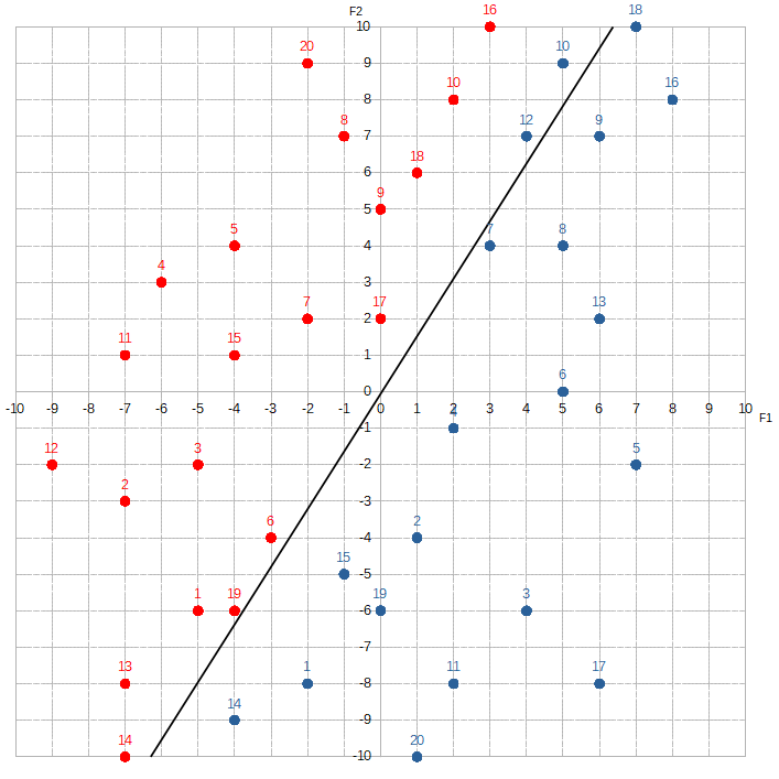
So the learning process basically boils down to simply moving this line around. That’s it. There’s no mystery whatsoever.
A bit underwhelming, isn’t it? To realize that moving a line around is what our own brains do all day … .
Let’s see how Alice does with the next data point ( F1 = -7, F2 = 3 ):
ptv2 = -0.60 * -7 + 0.38 * -3 + 0.02
ptv2 =     4.2    +  -1.14   + 0.02
ptv2 = 3.08
Since the predicted target value is positive, the masked target value equals 1, and Alice guesses the label is Hatfield.
TMfinal(  ) = ?

TM2(  ) = -0.60 * F1 + 0.38 * F2 + 0.020
Hatfield → ( masked ) target variable is 1
McCoy → ( masked ) target variable is -1
| Data Point | Feature 1 | Feature 2 | TM( ) Used | Predicted Target Variable | Masked Target Variable | Predicted Label | Target Variable | Label | Error |
|---|---|---|---|---|---|---|---|---|---|
| dpH1 | -5 | -6 | TM1() | -0.5 | -1 | McCoy | 1 | Hatfield | -2 |
| dpH2 | -7 | -3 | TM2() | 3.08 | 1 | Hatfield | 1 | Hatfield | 0 |
| etc. | etc. | etc. | … | … | … | … | etc. | etc. | … |
And the actual label is indeed Hatfield! Hooray! Alice got her first right answer!
She repeats these steps for the rest of the training set.
main(  )
{
    …

    repeat
    {
        dp = hvm.nextDataPoint;

        bob.collect_feature_value( dp.f1 );
        carol.collect_feature_value( dp.f2 );

        alice.collect_target_value( dp.trgtVal );
        alice.collect_label( dp.label );

        /* feedforward phase */
        alice.calc_predicted_target_val( friends );
        alice.calc_masked_target_val(  );
        alice.assign_predicted_label( "Hatfield", McCoy" );

        /* backpropagate phase */
        alice.calc_error( );
        alice.update_weights( friends );
    }

    …
}TMfinal( ) = ?
TM4( ) = -0.62 * F1 + 0.38 * F2 + -0.02Hatfield → ( masked ) target variable is 1
McCoy → ( masked ) target variable is -1
| Data Point | Feature 1 | Feature 2 | TM( ) Used | Predicted Target Variable | Masked Target Variable | Predicted Label | Target Variable | Label | Error |
|---|---|---|---|---|---|---|---|---|---|
| dpH1 | -5 | -6 | TM1() | -0.5 | -1 | McCoy | 1 | Hatfield | 2 |
| dpH2 | -7 | -3 | TM2() | 3.08 | 1 | Hatfield | 1 | Hatfield | 0 |
| … | … | … | … | … | … | … | … | … | … |
| dpM20 | 5 | 9 | TM4() | -4.44 | -1 | McCoy | -1 | McCoy | 0 |
| etc. | etc. | etc. | … | … | … | … | etc. | etc. | … |
Alright, let’s see how Alice did overall. We’ll calculate the total error — which is simply the sum of all the absolute values of the errors.
main( )
{
total_error;
…
repeat
{
dp = hvm.nextDataPoint;
bob.collect_feature_value( dp.f1 );
carol.collect_feature_value( dp.f2 );
alice.collect_target_value( dp.trgtVal );
alice.collect_label( dp.label );
/* feedforward phase */
alice.calc_predicted_target_val( friends );
alice.calc_masked_target_val( );
alice.assign_predicted_label( "Hatfield, McCoy" );
/* backpropagate phase */
alice.calc_error( );
alice.update_weights( friends );
}
total_error = sum( absolute_value( errors ) );
…
}Alice made a total error value of 6.0. Not bad for her first try!
Rinse N' Repeat
In the dart-throwing examples from previous posts, when we wanted to continue practicing, we simply threw more darts. Unfortunately, in this problem, we’ve run out of data points! So, how do we continue? Easy — we simply go back to the first data point. The difference now is that we use the more refined trained model, TM4( ), rather than the original, TM1( ).
TMfinal(  ) = ?

TM4(  ) = -0.62 * F1 + 0.38 * F2 + -0.02
Hatfield → ( masked ) target variable is 1
McCoy → ( masked ) target variable is -1
| Data Point | Feature 1 | Feature 2 | TM( ) Used | Predicted Target Variable | Masked Target Variable | Predicted Label | Target Variable | Label | Error |
|---|---|---|---|---|---|---|---|---|---|
| dpH1 | -5 | -6 | TM4() | 0.80 | 1 | Hatfield | 1 | Hatfield | 0 |
| etc. | etc. | etc. | … | … | … | … | etc. | etc. | … |
Since there’s always room for improvement, Alice can repeatedly iterate over this data set forever. But we don’t want that. We want her to stop at some point — so we’ll need to implement a couple of stopping conditions.
First, we’ll add a hard upper bound. This is the number of iterations that we’re pretty certain she will rarely need to reach. If she uses that many iterations, then chances are something went wrong in the learning process.
The other stopping condition will be the learning goal. A good spot to end would be when Alice predicts all the labels correctly. Any time prior to this means that she’s still making mistakes — which means there’s still more to learn. Once she gets all the labels right, however, she won’t learn anything new, so any additional studying would be useless.
main(  )
{
    iteration = 1;
    total_error;
    …

    repeat_until( iteration == 100 or total_error == 0.0 )
    {
        repeat
        {
            dp = hvm.nextDataPoint;

            bob.collect_feature_value( dp.f1 );
            carol.collect_feature_value( dp.f2 );

            alice.collect_target_value( dp.trgtVal );
            alice.collect_label( dp.label );

            /* feedforward phase */
            alice.calc_predicted_target_val( friends );
            alice.calc_masked_target_val(  );
            alice.assign_predicted_label( "Hatfield", "McCoy" );

            /* backpropagate phase */
            alice.calc_error( );
            alice.update_weights( friends );
        }

        total_error = sum( absolute_value( errors ) );
        iteration++;
    }

    …
}
Here are the end results:
TM10( ) = -0.68 * F1 + 0.38 * F2 + -0.14Hatfield → target variable is 1
McCoy → target variable is -1
| Data Point | Feature 1 | Feature 2 | TM( ) Used | Predicted Target Variable | Masked Target Variable | PredictedLabel | Target Variable | Label | Error |
|---|---|---|---|---|---|---|---|---|---|
| dpH1 | -5 | -6 | TM10() | 0.98 | 1 | Hatfield | 1 | Hatfield | 0 |
| dpH2 | -7 | -3 | TM10() | 3.48 | 1 | Hatfield | 1 | Hatfield | 0 |
| dpH3 | -5 | -2 | TM10() | 2.50 | 1 | Hatfield | 1 | Hatfield | 0 |
| dpH4 | -6 | 3 | TM10() | 5.08 | 1 | Hatfield | 1 | Hatfield | 0 |
| dpH5 | -4 | 4 | TM10() | 4.10 | 1 | Hatfield | 1 | Hatfield | 0 |
| dpH6 | -3 | -4 | TM10() | 0.38 | 1 | Hatfield | 1 | Hatfield | 0 |
| dpH7 | -2 | 2 | TM10() | 1.98 | 1 | Hatfield | 1 | Hatfield | 0 |
| dpH8 | -1 | 7 | TM10() | 3.20 | 1 | Hatfield | 1 | Hatfield | 0 |
| dpH9 | 0 | 5 | TM10() | 1.76 | 1 | Hatfield | 1 | Hatfield | 0 |
| dpH10 | 2 | 8 | TM10() | 1.54 | 1 | Hatfield | 1 | Hatfield | 0 |
| dpH11 | -7 | 1 | TM10() | 5.00 | 1 | Hatfield | 1 | Hatfield | 0 |
| dpH12 | -9 | -2 | TM10() | 5.22 | 1 | Hatfield | 1 | Hatfield | 0 |
| dpH13 | -7 | -8 | TM10() | 1.58 | 1 | Hatfield | 1 | Hatfield | 0 |
| dpH14 | -7 | -10 | TM10() | 0.82 | 1 | Hatfield | 1 | Hatfield | 0 |
| dpH15 | -4 | 1 | TM10() | 2.96 | 1 | Hatfield | 1 | Hatfield | 0 |
| dpH16 | 3 | 10 | TM10() | 1.62 | 1 | Hatfield | 1 | Hatfield | 0 |
| dpH17 | 0 | 2 | TM10() | 0.62 | 1 | Hatfield | 1 | Hatfield | 0 |
| dpH18 | 1 | 6 | TM10() | 1.46 | 1 | Hatfield | 1 | Hatfield | 0 |
| dpH19 | -4 | -6 | TM10() | 0.30 | 1 | Hatfield | 1 | Hatfield | 0 |
| dpH20 | -2 | 9 | TM10() | 4.64 | 1 | Hatfield | 1 | Hatfield | 0 |
| dpM1 | -2 | -8 | TM10() | -1.82 | -1 | McCoy | -1 | McCoy | 0 |
| dpM2 | 1 | -4 | TM10() | -2.34 | -1 | McCoy | -1 | McCoy | 0 |
| dpM3 | 4 | -6 | TM10() | -5.14 | -1 | McCoy | -1 | McCoy | 0 |
| dpM4 | 2 | -1 | TM10() | -1.88 | -1 | McCoy | -1 | McCoy | 0 |
| dpM5 | 7 | -2 | TM10() | -5.66 | -1 | McCoy | -1 | McCoy | 0 |
| dpM6 | 5 | 0 | TM10() | -3.54 | -1 | McCoy | -1 | McCoy | 0 |
| dpM7 | 3 | 4 | TM10() | -0.66 | -1 | McCoy | -1 | McCoy | 0 |
| dpM8 | 5 | 4 | TM10() | -2.02 | -1 | McCoy | -1 | McCoy | 0 |
| dpM9 | 6 | 7 | TM10() | -1.56 | -1 | McCoy | -1 | McCoy | 0 |
| dpM10 | 5 | 9 | TM10() | -0.12 | -1 | McCoy | -1 | McCoy | 0 |
| dpM11 | 2 | -8 | TM10() | -4.54 | -1 | McCoy | -1 | McCoy | 0 |
| dpM12 | 4 | 7 | TM10() | -0.20 | -1 | McCoy | -1 | McCoy | 0 |
| dpM13 | 6 | 2 | TM10() | -3.46 | -1 | McCoy | -1 | McCoy | 0 |
| dpM14 | -4 | -9 | TM10() | -0.84 | -1 | McCoy | -1 | McCoy | 0 |
| dpM15 | -1 | -5 | TM10() | -1.36 | -1 | McCoy | -1 | McCoy | 0 |
| dpM16 | 8 | 8 | TM10() | -2.54 | -1 | McCoy | -1 | McCoy | 0 |
| dpM17 | 6 | -8 | TM10() | -7.26 | -1 | McCoy | -1 | McCoy | 0 |
| dpM18 | 7 | 10 | TM10() | -1.10 | -1 | McCoy | -1 | McCoy | 0 |
| dpM19 | 0 | -6 | TM10() | -2.42 | -1 | McCoy | -1 | McCoy | 0 |
| dpM20 | 1 | -10 | TM10() | -4.62 | -1 | McCoy | -1 | McCoy | 0 |
Let’s test Alice’s new found knowledge with some test data ( the grey dots ).
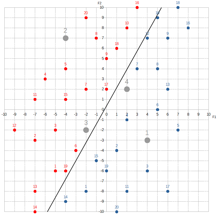
TM10( ) = -0.68 * F1 + 0.38 * F2 + -0.14Hatfield → ( masked ) target variable is 1
McCoy → ( masked ) target variable is -1
| Data Point | Feature 1 | Feature 2 | TM( ) Used | Predicted Target Variable | Masked Target Variable | Predicted Label | Target Variable | Label | Correct? |
|---|---|---|---|---|---|---|---|---|---|
| dpT1 | 4 | -3 | TM10() | -4 | -1 | McCoy | -1 | McCoy | Yes! |
| dpT2 | -4 | 7 | TM10() | 5.24 | 1 | Hatfield | 1 | Hatfield | Yes! |
| dpT3 | -2 | -2 | TM10() | 0.46 | 1 | Hatfield | 1 | Hatfield | Yes! |
| dpT4 | 2 | 2 | TM10() | -0.74 | -1 | McCoy | -1 | McCoy | Yes! |
Not too bad!
Here’s the code we have:
main(  )
{
    iteration = 1;
    total_error;

    alice = new OutputNeuron(  );
    bob = new InputNeuron(  );
    carol = new InputNeuron(  );

    friends = { bob, carol };

    hvm = new SyntheticData(  );
    hvm.collect_data
        ( "train_hatfields_vs_mccoys.txt" );

    repeat_until( iteration == 100 or total_error == 0.0 )
    {
        repeat
        {
            dp = hvm.nextDataPoint;

            bob.collect_feature_value( dp.f1 );
            carol.collect_feature_value( dp.f2 );

            alice.collect_target_value( dp.trgtVal );
            alice.collect_label( dp.label );

            /* feedforward phase */
            alice.calc_predicted_target_val( friends );
            alice.calc_masked_target_val(  );
            alice.assign_predicted_label
                ( "Hatfield", "McCoy" );

            /* backpropagate phase */
            alice.calc_error( );
            alice.update_weights( friends );
        }

        total_error = sum( absolute_value( errors ) );
        iteration++;
    }

    /* final exam */
    numCorrectAnswers = 0;
    numWrongAnswers = 0;
    hvmTest = new SyntheticData(  );
    hvmTest.collect_data
        ( "test_hatfields_vs_mccoys.txt" );

    repeat
    {
        dp = hvmTest.nextDataPoint;
        bob.collect_feature_value( dp.f1 )
        carol.collect_feature_value( dp.f2 );

        /* feedforward phase ONLY */
        alice.calc_predicted_target_val( friends );
        alice.calc_masked_target_val(  );
        alice.assign_predicted_label( "Hatfield", "McCoy" );

        if ( alice.maskedTrgtVal == dp.trgtVal )
            numCorrectAnswers++;
        else
            numWrongAnswers++
    }

    …
}
/* separate source file */
class OutputNeuron
{
learningRate = 0.01;
trgtVal;
label;
bias;
prdctdTrgtVal;
maskedTrgtVal;
prdctdLabel;
error = 0;
set_bias( value )
{
bias = value;
}
collect_target_value( value )
{
trgtVal = value;
}
collect_label( value )
{
label = value;
}
calc_predicted_target_val( inputNeurons )
{
collect_feature_values_from( inputNeurons );
collect_weights_from( inputNeurons );
prdctdTrgtVal = sum( weights * features ) + bias;
}
calc_masked_target_val( )
{
if ( prdctdTrgtVal > 0 )
maskedTrgtVal = 1;
else
maskedTrgtVal = -1;
}
assign_predicted_label( lbl1, lbl2 )
{
if ( maskedTrgtVal = 1 )
prdctdLabel = lbl1;
else
prdctdLabel = lbl2;
}
collect_feature_values_from( inputNeurons )
{ … }
collect_weights_from( inputNeurons );
{ … }
calc_error( )
{
if ( maskedTrgtVal ≠ trgrtVal )
error = maskedTrgtVal - trgtVal;
}
update_weights( inputNeurons )
{
foreach neuron in inputNeurons
{
neuron.weight.add( error * neuron.featureVals *
learningRate );
}
bias.add( error * learningRate );
}
…
}/* separate source file */
class SyntheticData
{
collect_data( filename )
{ … }
…
}/* separate source file */
class InputNeuron
{
feature;
weight;
collect_feature_value
( value )
{
feature = value;
}
set_weight( value )
{
weight = value;
}
…
}I Have A Face For Radio
Alright, enough with these silly pen-n-paper-based toy problems. Let’s give Alice a problem that is much more like the ones that real-world machine learning systems tackle. She’s going to recognize faces!
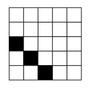
But I need to confess — new technology scares the living crap out of me. So, instead of using the latest digital camera — with their terrifying 50 megapixels and 16 million colors — we’re going to use the original digital camera that Thomas Edison himself invented. It takes black-&-white 5 x 5 photos, for a whopping total of 25 pixels. Call me old fashioned, but I don’t need rich details nor vibrant colors. Those things belong in salads — not photographs.
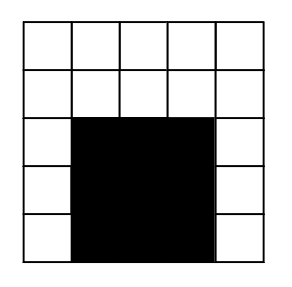
Here’s a picture of your friend:
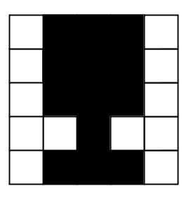
Oh my, she’s quite photogenic!
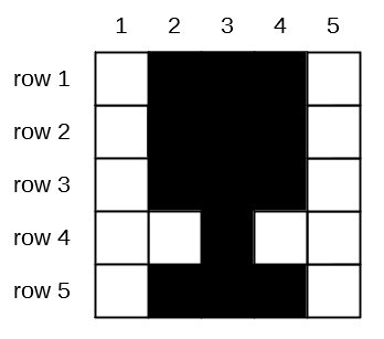
We’re going to have Alice try to distinguish between your friend and a french fry:
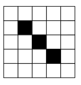
I know it’s hard to tell which is which. The differences are quite subtle — but if you look closely, you’ll notice that your friend’s face is three pixels wide, while the fry is only one pixel wide. Plus, the fry doesn’t have a neck nor shoulders like your friend does. Alice will try to learn these differences.
If we label each row of the pictures as 1, 2, 3, 4, & 5 from the top down, and the columns as 1, 2, 3, 4, & 5 from left to right, we can “flatten” each picture into a single line:
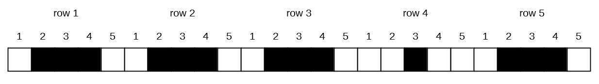
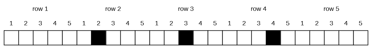
If we also assign all the black pixels the number 1 and the white pixels the number -1, we can put these photographs into our usual table format:
TM( ) = ?friend → target variable is 1
fry → target variable is -1
| Photo | Pixel (1, 1) | Pixel (1, 2) | Pixel (1, 3) | Pixel (1, 4) | Pixel (1, 5) | Pixel (2, 1) | Pixel (2, 2) | Pixel (2, 3) | Pixel (2, 4) | Pixel (2, 5) | Pixel (3, 1) | Pixel (3, 2) | Pixel (3, 3) | Pixel (3, 4) | Pixel (3, 5) | Pixel (4, 1) | Pixel (4, 2) | Pixel (4, 3) | Pixel (4, 4) | Pixel (4, 5) | Pixel (5, 1) | Pixel (5, 2) | Pixel (5, 3) | Pixel (5, 4) | Pixel (5, 5) | Target Variable | Label |
|---|---|---|---|---|---|---|---|---|---|---|---|---|---|---|---|---|---|---|---|---|---|---|---|---|---|---|---|
| photo1 | -1 | 1 | 1 | 1 | -1 | -1 | 1 | 1 | 1 | -1 | -1 | 1 | 1 | 1 | -1 | -1 | -1 | 1 | -1 | -1 | -1 | 1 | 1 | 1 | -1 | 1 | friend |
| photo2 | -1 | -1 | -1 | -1 | -1 | -1 | 1 | -1 | -1 | -1 | -1 | -1 | 1 | -1 | -1 | -1 | -1 | -1 | 1 | -1 | -1 | -1 | -1 | -1 | -1 | -1 | fry |
Each data point represents a single photograph, and each feature represents a single pixel.
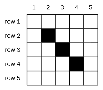
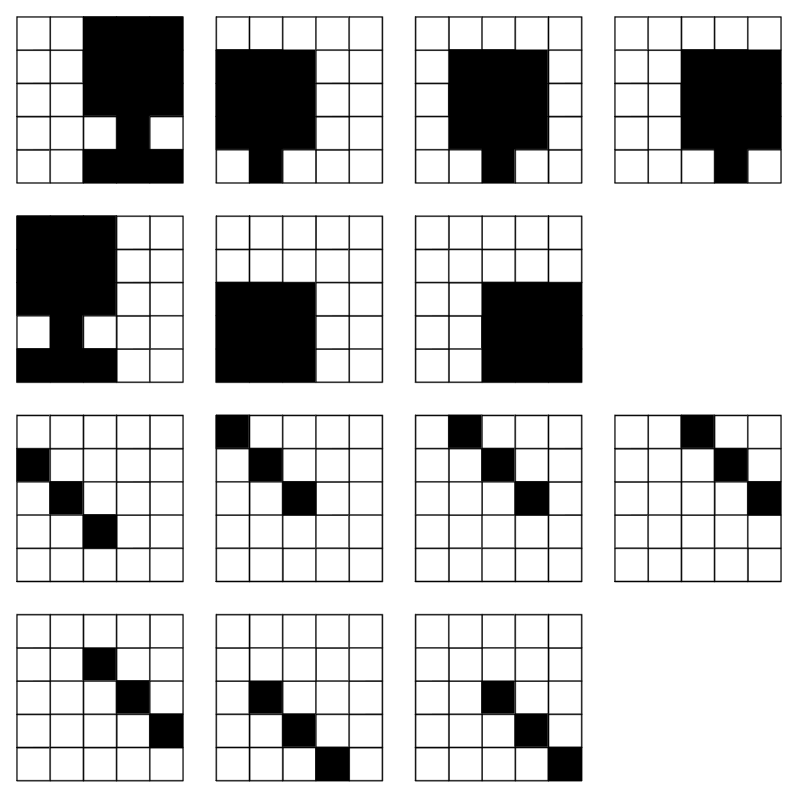
Here are more photos of your friend and of the fry:
TM( ) = ?friend → target variable is 1
fry → target variable is -1
| Photo | Pixel (1, 1) | Pixel (1, 2) | Pixel (1, 3) | Pixel (1, 4) | Pixel (1, 5) | Pixel (2, 1) | Pixel (2, 2) | Pixel (2, 3) | Pixel (2, 4) | Pixel (2, 5) | Pixel (3, 1) | Pixel (3, 2) | Pixel (3, 3) | Pixel (3, 4) | Pixel (3, 5) | Pixel (4, 1) | Pixel (4, 2) | Pixel (4, 3) | Pixel (4, 4) | Pixel (4, 5) | Pixel (5, 1) | Pixel (5, 2) | Pixel (5, 3) | Pixel (5, 4) | Pixel (5, 5) | Target Variable | Label |
|---|---|---|---|---|---|---|---|---|---|---|---|---|---|---|---|---|---|---|---|---|---|---|---|---|---|---|---|
| photo1 | -1 | 1 | 1 | 1 | -1 | -1 | 1 | 1 | 1 | -1 | -1 | 1 | 1 | 1 | -1 | -1 | -1 | 1 | -1 | -1 | -1 | 1 | 1 | 1 | -1 | 1 | friend |
| photo2 | -1 | -1 | -1 | -1 | -1 | -1 | 1 | -1 | -1 | -1 | -1 | -1 | 1 | -1 | -1 | -1 | -1 | -1 | 1 | -1 | -1 | -1 | -1 | -1 | -1 | -1 | fry |
| photo3 | 1 | 1 | 1 | -1 | -1 | 1 | 1 | 1 | -1 | -1 | 1 | 1 | 1 | -1 | -1 | -1 | 1 | -1 | -1 | -1 | 1 | 1 | 1 | -1 | -1 | 1 | friend |
| photo4 | -1 | -1 | 1 | 1 | 1 | -1 | -1 | 1 | 1 | 1 | -1 | -1 | 1 | 1 | 1 | -1 | -1 | -1 | 1 | -1 | -1 | -1 | 1 | 1 | 1 | 1 | friend |
| photo5 | -1 | -1 | -1 | -1 | -1 | 1 | 1 | 1 | -1 | -1 | 1 | 1 | 1 | -1 | -1 | 1 | 1 | 1 | -1 | -1 | -1 | 1 | -1 | -1 | -1 | 1 | friend |
| photo6 | -1 | -1 | -1 | -1 | -1 | -1 | 1 | 1 | 1 | -1 | -1 | 1 | 1 | 1 | -1 | -1 | 1 | 1 | 1 | -1 | -1 | -1 | 1 | -1 | -1 | 1 | friend |
| photo7 | -1 | -1 | -1 | -1 | -1 | -1 | -1 | 1 | 1 | 1 | -1 | -1 | 1 | 1 | 1 | -1 | -1 | 1 | 1 | 1 | -1 | -1 | -1 | 1 | -1 | 1 | friend |
| photo8 | -1 | -1 | -1 | -1 | -1 | -1 | -1 | -1 | -1 | -1 | 1 | 1 | 1 | -1 | -1 | 1 | 1 | 1 | -1 | -1 | 1 | 1 | 1 | -1 | -1 | 1 | friend |
| photo9 | -1 | -1 | -1 | -1 | -1 | -1 | -1 | -1 | -1 | -1 | -1 | -1 | 1 | 1 | 1 | -1 | -1 | 1 | 1 | 1 | -1 | -1 | 1 | 1 | 1 | 1 | friend |
| photo10 | -1 | -1 | -1 | -1 | -1 | -1 | -1 | 1 | -1 | -1 | -1 | -1 | -1 | 1 | -1 | -1 | -1 | -1 | -1 | 1 | -1 | -1 | -1 | -1 | -1 | -1 | fry |
| photo11 | -1 | 1 | -1 | -1 | -1 | -1 | -1 | 1 | -1 | -1 | -1 | -1 | -1 | 1 | -1 | -1 | -1 | -1 | -1 | -1 | -1 | -1 | -1 | -1 | -1 | -1 | fry |
| photo12 | -1 | -1 | 1 | -1 | -1 | -1 | -1 | -1 | 1 | -1 | -1 | -1 | -1 | -1 | 1 | -1 | -1 | -1 | -1 | -1 | -1 | -1 | -1 | -1 | -1 | -1 | fry |
| photo13 | 1 | -1 | -1 | -1 | -1 | -1 | 1 | -1 | -1 | -1 | -1 | -1 | 1 | -1 | -1 | -1 | -1 | -1 | -1 | -1 | -1 | -1 | -1 | -1 | -1 | -1 | fry |
| photo14 | -1 | -1 | -1 | -1 | -1 | -1 | -1 | -1 | -1 | -1 | -1 | 1 | -1 | -1 | -1 | -1 | -1 | 1 | -1 | -1 | -1 | -1 | -1 | 1 | -1 | -1 | fry |
| photo15 | -1 | -1 | -1 | -1 | -1 | -1 | -1 | -1 | -1 | -1 | -1 | -1 | 1 | -1 | -1 | -1 | -1 | -1 | 1 | -1 | -1 | -1 | -1 | -1 | 1 | -1 | fry |
| photo16 | -1 | -1 | -1 | -1 | -1 | 1 | -1 | -1 | -1 | -1 | -1 | 1 | -1 | -1 | -1 | -1 | -1 | 1 | -1 | -1 | -1 | -1 | -1 | -1 | -1 | -1 | fry |
Okay, this task is almost the same as the previous one. The only difference is that in the previous problem, Alice had to find a one-dimensional line that bisected the two-dimensional featurespace in a such way that organized all the Hatfields on one side of the line and the McCoys on the other. In this facial recognition problem, Alice needs to find a 24-dimensional hyperplane that bisects the 25-dimensional featurespace such that the photos of your friend fall on one side of the hyperplane and the photos of the fry fall on the other. It’s impossible for me to draw a 24-dimensional hyperplane in a 25-dimensional featurespace, so you’ll need to use your imagination.
And no, I do not have the budget to rent out a couple of giant data centers to do the imagining for you.
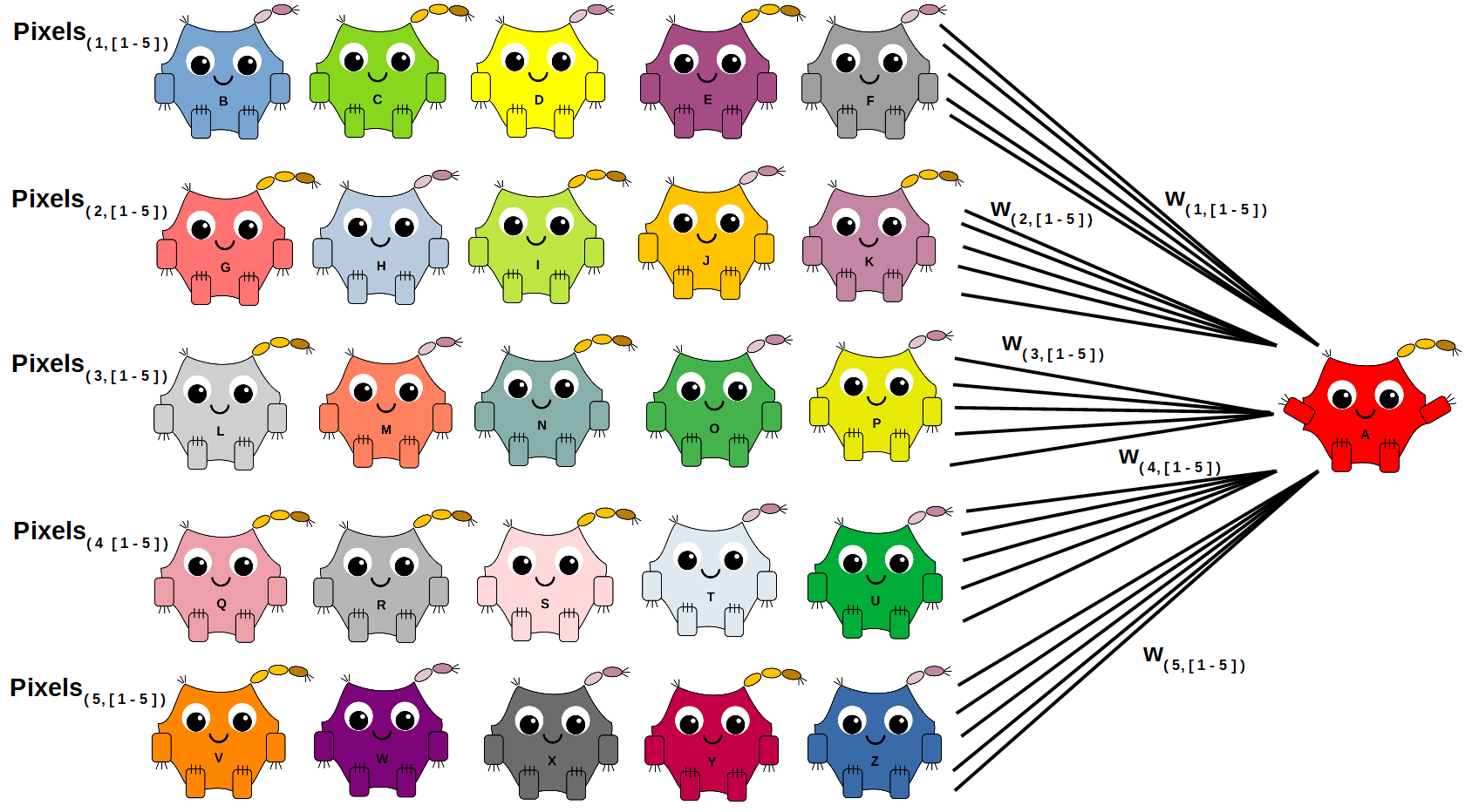
However, because Alice and her friends were created only moments ago, we do need to be mindful about overwhelming them. What’s the solution? Well, since the Build-A-Neuron Workshop is open til ten o’clock, let make her some more friends!
main( )
{
    …

    faceData = new SyntheticData( );
    faceData.retrieve_data( "train_face_recognition.txt" );

    deke = new InputNeuron( );
    echo = new InputNeuron( );
    foxtrot = new InputNeuron( );
    gamma = new InputNeuron( );
    hank = new InputNeuron( );
    igloo = new InputNeuron( );
    jacob = new InputNeuron( );
    katie = new InputNeuron( );
    lima = new InputNeuron( );
    mack = new InputNeuron( );
    nancy = new InputNeuron( );
    opie = new InputNeuron( );
    pedro = new InputNeuron( );
    quirky = new InputNeuron( );
    robin = new InputNeuron( );
    silly = new InputNeuron( );
    toby = new InputNeuron( );
    unique = new InputNeuron( );
    violet = new InputNeuron( );
    wilco = new InputNeuron( );
    xray = new InputNeuron( );
    yankee = new InputNeuron( );
    zulu = new InputNeuron( );

    friends.add( { deke, echo, foxtrot, gamma, hank, igloo, jacob,
                   katie, lima, mack, nancy, opie, pedro, quirky,
                   robin, silly, toby, unique, violet, wilco, xray,
                   yankee, zulu } );

    …
}
Goodness, this is starting to look like a Saturday morning cartoon!
After iterating through the training data several times, Alice arrives at this trained model: TM16( ) = 0.128 * F1 + 0.596 * F2 + 0.086 * F3 + -0.077 * F4 + 0.464 * F5 + -0.139 * F6 + 0.775 * F7 + 0.455 * F8 + 0.737 * F9 + 0.350 * F10 + 0.457 * F11 + 0.485 * F12 + 1.091 * F13 + 0.076 * F14 + 0.801 * F15 + 0.854 * F16 + 0.761 * F17 + 0.864 * F18 + 0.883 * F19 + 0.325 * F20 + 0.241 * F21 + 0.425 * F22 + 0.653 * F23 + 0.689 * F24 + 0.420 * F25 + 1.108.
Let’s test her new found skill with two test photos:
TM16( ) = 0.128 * F1 + 0.596 * F2 + 0.086 * F3 + -0.077 * F4 + 0.464 * F5 + -0.139 * F6 + 0.775 * F7 + 0.455 * F8 + 0.737 * F9 + 0.350 * F10 + 0.457 * F11 + 0.485 * F12 + 1.091 * F13 + 0.076 * F14 + 0.801 * F15 + 0.854 * F16 + 0.761 * F17 + 0.864 * F18 + 0.883 * F19 + 0.325 * F20 + 0.241 * F21 + 0.425 * F22 + 0.653 * F23 + 0.689 * F24 + 0.420 * F25 + 1.108friend → ( masked ) target variable is 1
fry → ( masked ) target variable is -1
| Photo | Pixel (1, 1) | Pixel (1, 2) | Pixel (1, 3) | Pixel (1, 4) | Pixel (1, 5) | Pixel (2, 1) | Pixel (2, 2) | Pixel (2, 3) | Pixel (2, 4) | Pixel (2, 5) | Pixel (3, 1) | Pixel (3, 2) | Pixel (3, 3) | Pixel (3, 4) | Pixel (3, 5) | Pixel (4, 1) | Pixel (4, 2) | Pixel (4, 3) | Pixel (4, 4) | Pixel (4, 5) | Pixel (5, 1) | Pixel (5, 2) | Pixel (5, 3) | Pixel (5, 4) | Pixel (5, 5) | Predicted Target Variable | Masked Target Variable | Predicted Label | Target Variable | Label | Correct? |
|---|---|---|---|---|---|---|---|---|---|---|---|---|---|---|---|---|---|---|---|---|---|---|---|---|---|---|---|---|---|---|---|
| photo17 | -1 | -1 | -1 | -1 | -1 | -1 | -1 | -1 | -1 | -1 | -1 | 1 | 1 | 1 | -1 | -1 | 1 | 1 | 1 | -1 | -1 | 1 | 1 | 1 | -1 | 0.561 | 1 | friend | 1 | friend | Yes! |
| photo18 | -1 | -1 | -1 | -1 | -1 | -1 | -1 | -1 | -1 | -1 | 1 | -1 | -1 | -1 | -1 | -1 | 1 | -1 | -1 | -1 | -1 | -1 | 1 | -1 | -1 | -7.548 | -1 | fry | -1 | fry | Yes! |
Not bad!
Warning:  Curves Ahead
Alice was able to find the appropriate trained models for the above two problems because the datasets were linearly separable. This simply means you can draw a straight line ( or an ( n – 1 )-dimensional hyperplane ) through the dataset that completely separates one group of points with the same label from another group of points with a different label.
If the points are situated in a way that only curved lines can bisect them, then Alice will never find a solution — since no linear solution exists!
Even worse is if some of the Hatfields and the McCoys are intermingled in a Romeo-and-Juliet-type tragedy. Then no simple function can successfully bisect the training set without mislabeling at least some of the data points.
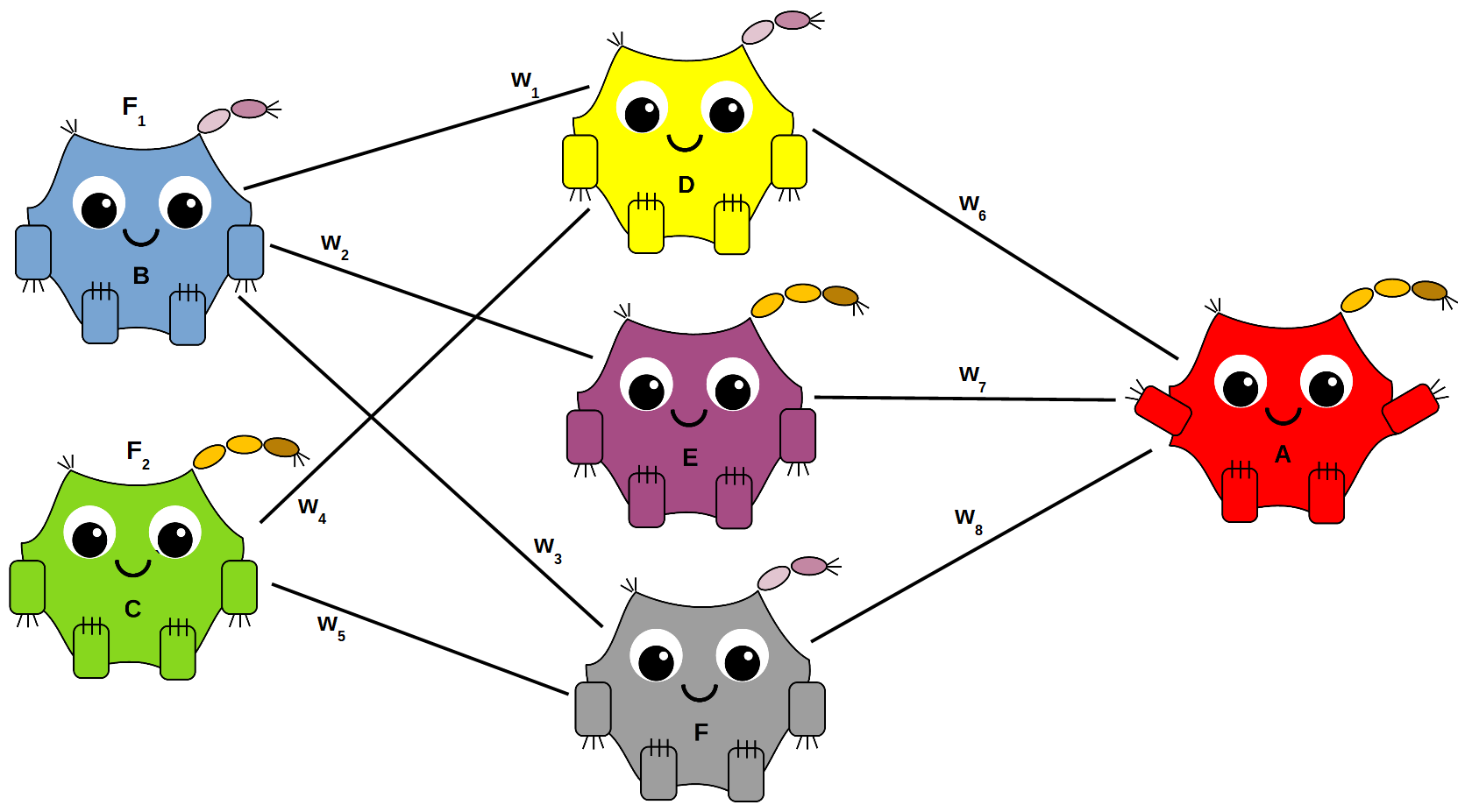
To deal with these kinds of complicated problems, you would need to use a more complicated neural network — one that contains more than just an input neural layer and an output neural layer. It would need additional hidden layers. These layers can take the inputs and combine them in different ways to make things as complicated as you need them to be. The following shows Deke, Echo, and Foxtrot forming a hidden layer.
Dart throwing is an example of a non-linearly separable problem. Rather than a straight line, you would need to find a circle, w1*F12 + w2*F22 + w0 = 0, that carves out the featurespace so that the BULLSEYE data points are separated from the NOT_BULLSEYE data points.
Okay, technically, you can tweak the inputs in such a way that would transform this problem from a circular regression to a linear regression that Alice can handle. I’ll leave that as an exercise for you to figure out. ( Here’s a hint: the circle equation, w1*F12 + w2*F22 + w0, looks a lot like the line equation, w1*F1 + w2*F2 + w0 — except that F1 and F2 are squared. So, … . )
Activation Functions
The step function used for masking the predicted target value is known as an activation function. The reason it’s called an activation function is because it makes our artificial neuron behave like a real neuron. A biological neuron normally is in a default state that emits a low-level signal. In our case, this state refers to the lower masked target value — -1. An activation function defines the conditions that would “activate” the neuron to go into a higher, more excited state that would emit a stronger signal. Thus, the step function tells Alice to “fire” a 1 whenever the predicted target value is positive.
Activation functions come in many shapes and sizes. The four most common are:
Step:
maskedTV = 1 if predictedTV is positive,
           -1 otherwise
Sigmoid:
maskedTV = 1 / ( 1 + e-predictedTV )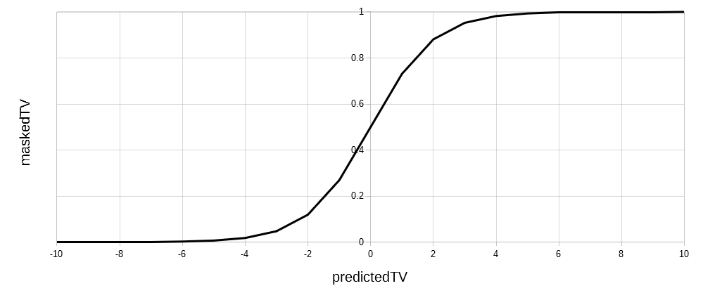
Tanh:
maskedTV = ( e2*predictedTV - 1 ) / ( e2*predictedTV + 1 )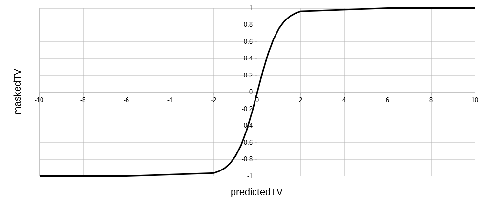
Rectified Linear Unit ( ReLU ):
maskedTV = predictedTV if positive,
           0 otherwise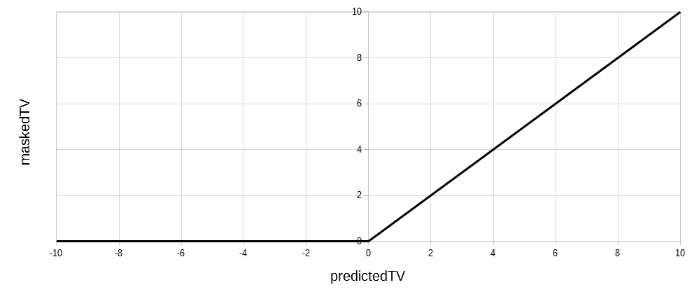
‘e‘ stands for the Euler number, which is a constant that approximately equals 2.7182. Sigmoid and tanh functions are similar to the step function, except that rather than a sudden jump from the low to high state, the transition starts slowly before gaining steam.
Activation functions serve numerous purposes. The top three reasons are:
- to simplify computation
- to improve predictive accuracy
- to manage structural problems
The first two reasons were why Alice used the step function.
An example of the third reason would be when using a leaky version of the ReLU function. Certain learning problems can cause neurons to “die”. For whatever reason, a weight may get reduced to zero, or the neuron may act a bit hinky — resulting in only outputting zeros. This essentially means it stops transmitting any information and is considered “dead”. This oftentimes can cascade over to subsequent layers — to the point where whole regions of a neural network would just shut off.
The leaky ReLU is like the regular ReLU, except that the negative predicted target values are masked with either a small nonzero constant or some fraction of the predicted value. This forces the neuron to always transmit a tiny pulse, which minimizes the risk of “dying”.
Leaky ReLU:
maskedTV = predictedTV if positive,
           a * predictedTV otherwise, where a is a fraction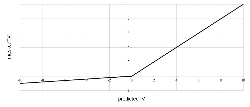
Attention Shoppers, The Build-A-Neuron Workshop  Will Be closing in Fifteen Minutes
Oh my, how time flies! I hope you had fun. Once you’ve paid at the checkout counter, you can pick up your neurons here.
The link contains a working version of the code and is written in Java. You should download it and run it to see how Alice and her awesome friends work!
Thank you so much for coming! We really appreciate your patronage and hope to see you again soon!

A good analogy would be to think of Alice as the President of the United States, and her friends as members of her cabinet. They provide her with the information she needs to make critical decisions.
Alice: “Alright, everyone, I need ideas! We’re facing a national french fries shortage! What the heck is going on?”
Hank: “Well, as the head of Homeland Security, I say we send in our best counter-terrorism expert, Jack Bauer, to get to the bottom of this. I hear fries factories are filled with lamps and electrical cords, so he should have plenty of tools to ‘enhanced-interrogate’ the workers.”
Alice: “Geez, Hank, your solution to everything is to trot out that psychopath. You know what — I’m downgrading your weight. You’re like a hammer that thinks every problem is a frickin’ nail!”
Hank: “But, ma’am, you do that, and the terrorists win!”
Alice: “Then so be it. Carol, you’re the commerce secretary. What do you think?”
Carol: “Well, I didn’t enhanced-interrogate anyone, but I did speak to the CEOs of all the major fries-making companies, and they tell me it’s a supply chain issue. They’re having a difficult time securing enough potatoes — all because of this new potato light bulb craze.”
Alice: “Potato light bulb craze?”
Carol: “Yeah, ever since a video went viral of some guy powering a light bulb with a potato, everyone has gone nuts with rewiring their homes to run on spuds — from dishwashers to air conditioners. I haven’t seen this kind of insanity since the Garbage Pail Kids trading card mania during the 1980s! Mack, you’re the Agricultural Secretary. Any word from the potato industry?”
Mack: “Yes, I’ve spoken to numerous potato farmers’ associations across the country, and they all tell me they’re trying their best to meet the spike in demand. They estimate it’ll take them about four months to ramp up their production sufficiently.”
Echo: “As the head of the Health and Human Services department, I am deeply concerned that four months will be too late.”
Alice: “Why?”
Echo: “By then most Americans will have turned to healthier alternatives — like celery stalks and carrot sticks. Once they start eating those bland things, they will never, ever return to yummy, delicious fries.”
Alice: “Good God! Forget the terrorists! If Americans start eating healthy, then the commies win! NOT GONNA HAPPEN ON MY WATCH!”
Deke: “Ms. President, as Defense Secretary, I may have a solution — but there’s a risk you won’t like.”
Alice: “I’m listening.”
Deke: “We can open up our national fries reserves and have the military air drop payloads of fries into every major metropolitan area — until the potato farmers can shore up their output. We should have enough in the reserves to last for more than six months.”
Mack: “What type of fries do we have?”
Deke: “Steak fries, curly fries, crinkle-cut fries — you name it, we’ve got it. We even have hash browns and tater tots.”
Mack: “NOICE!”
Alice: “That’s a fantastic idea! But what’s the downside?”
Deke: “Well, dropping heavy supplies into densely-populated urban centers is extremely dangerous. Civilians may get killed.”
Echo: “Oh, I guarantee that that WILL happen. There be like some really stupid people out there who’ll want to be the first to sink their teeth into those fries. They’ll run under the pallets and get squashed like bugs! This has the makings of a PR nightmare.”
Alice: “Dammit, this is a national emergency! We’ll just have to deal with it if and when that happens. Alright, neurons, let’s make Operation Freedom Fries a go!”
They grow up so fast, don’t they? One minute, they just want a hug — the next, they’re running the country!
Footnote
Here are some additional fascinating articles about neural networks:
- Deep Neural Networks Help to Explain Living Brains
- Job One for Quantum Computers: Boost Artificial Intelligence — discusses the possibility of using quantum mechanics and quantum computing to improve artificial neural networks